Video "Lessons from the Peloton"

I've prepared an 8 minute video Lessons from the Peloton  in which I discuss the concept of group sorting and phase transitions in pelotons. I show my own footage of various bicycle races, flocks, non-biological systems, and other kinds of human organizations.  It's a "popular" video, which I've actually entered as a submission to the Vancouver Island Short Film Festival.  As an amateur videographer, I don't have a good sense of its chances in making it into the festival, but whether the video gets into the festival or not, it helps to explain in a non-technical way some of my own work and interest in the behavior of pelotons.

Peloton Anatomy - some updates

Following on an earlier post about sorting dynamics, here I recap generally a few developments with some short demonstrations.

I've incorporated a deceleration algorithm that allows us to show how much a following cyclist needs to decelerate in order to stay at or below his/her threshold if a leading cyclist drives the speed of the peloton too high for the following cyclist. This is a significant development over previous models, one of mine, and one by Erick Ratamero.  Basically, I've incorporated the new deceleration algorithm into Ratamero's model, for a new model.

Ratamero's model is still sound because it models cyclists' overall energy expenditure in peloton conditions, while this new model allows us to see changing peloton dynamics as group speeds change throughout the course of a race. Nor is my earlier model invalidated, since it applied the same basic principle I use in the new model, except that the old model did not apply any actual speed, power or MSO data. That said, while I could defend the basic principles of my old model, we can now essentially discard it in favor of this new model.

To demonstrate the new model, first take a look at the link below of accelerated footage of the 2013 BC Championships women's Points Race. Pay attention to the oscillations between stretching (single-file) and compact formations. The accelerated motion of the video is about 2X normal speed. I hope the "Ride of the Valkyries" background music isn't too distracting!

 Points race - accelerated

Keeping the dynamics of that race in mind, below is a simulated version of the same race, accelerated to about twice as fast again so you can see the whole race occur in a short time. I've incorporated the speed parameters that I derived at two timing places per lap, and encoded it into the simulation.You can see the speed changes according to the power graph to the lower right. When the power output spikes, you can see certain cyclists are forced to decelerate relative to others. When the speed relaxes, the peloton reintegrates and its density increases.  This relaxation oscillation is well modeled by the new algorithm.

The numbers you see on the "backs" of the riders are their "maximal sustainable outputs" (MSOs), or their maximal sustainable power for a duration between 30 seconds and 5 minutes. These are derived from the cyclists' 200m sprint times, and multiplied by a value that reflects their sustained maximum output during the race for between 30s and 5 minutes.

simulated peloton 14 cyclists

With that fairly accurate simulation, we can try some experiments. For example, we can increase the size of the peloton.  Here is a view of 50 cyclists with the same speed profile as for the 14 cyclists above.

simulated peloton 50 cyclists

Now let's take a look at 100 cyclists (link below).  I've only included part of the video here, since the simulation runs slower with 100 cyclists, and the point is made with a slightly abbreviated version.  Quite a bit more impressive, though, to see a much larger group and its dynamics, using the same speed profile as for the original 14 cyclists. What is interesting with 100 cyclists, which is not so easy to see with smaller the simulated pelotons, is that in the position profile graph we can see some evidence of the "convection" dynamic that I have spoken of in previous posts.  It seems that it may be a dynamic that only clearly emerges at some threshold peloton size and speed.  You can see this somewhat for 50 cyclists, but still it seems clearer in runs of 100 cyclists.

 simulated peloton 100 cyclists

I am looking to have the new model published (with the same three collaborators on our last published paper: Richardson, Ratamero, Perc). In this new paper, we will show how the model demonstrates sorting of the peloton into groups, and some results to this effect.

In future, we still need to investigate and report more definitively on the convection dynamic. So that could be the subject of the next paper - or I am also interested in obtaining  some more evidence of the hysteresis effect I observed a few years ago, and presented in principle at an AAAI conference.

I'm also now interested in developing a peloton solution to the tragedy of the commons (ToC),  having been somewhat inspired by Francis Heylighen's recent efforts to show a self-organized solution to the ToC (not yet published).

Of course there is also some fluid dynamics analogies I want to develop, and recently I have been thinking about Stokes Law and particle settling as somewhat analagous to peloton sub-group sorting. Is there some sort of equivalency between the size of a particle moving through fluid, and the MSO of a rider?

Calibrating the simulation

Having made a few adjustments to the newest peloton simulation model, I have produced an excellent simulation result of the women's 2013 BC Championships Points race. 

Figure 1 is a graph of the actual position data from the women's Points race.  There were 14 riders in the race.

Figure 1. Position data from 2013 women's Points race, BC Championships.

In the Netlogo model, I set 14 simulated riders with maximal-sustainable-outputs (MSOs) corresponding to those of the women in the race*.  Using the speed data from that race, I inputted the speeds in the appropriate time sequence into the simulation, corresponding to power values in the second graph from the top in Figure 2 below. This generated the position graph (top graph below). The similarities are quite remarkable, and this is good evidence that the new model is solid.

    

Figure 2.  Simulation results using data from women's Points race.  14 riders with MSOs corresponding to 200m sprint times. Speeds were input according to data (indicated by power graph), and the outputs are shown by the position graph, PCR, and peloton stretch. Peloton stretch is the distance from the front rider to the rear rider, indicating changing length of the peloton.

*I used the 200m sprint times as the starting point for these. There were three riders in the points race who did not race the 200m TT, and so I used the mean of the other 11 for the missing ones in the simulation.

short addendum to "Peloton Sorting" post

I've ironed out a small problem that revealed itself in the PCR graphs in the last post.  There were some anomalous downward spikes in PCR values which indicated a problem. I've located the source of that problem, and can show that this has been fixed. 

Below are two updated samples to show this. Both graphs show mean PCR values in black, and a random cyclist in green. I've manually varied power-output factors at random times. 

In the top one, the sample cyclist exhibits values above the mean, which means that he/she is weaker than the mean (higher PCR means cyclist approaches threshold); while the second shows the sample cyclist PCR values generally below the mean. The troubling downward spikes are eliminated.  There is no concern that PCR values show >1, as these represent the effective values at the speed (or grade, wind-speed) selected. 

Peloton sorting dynamics

Building on Erick Ratamero's MOPED peloton model [1], and introducing a number of new elements based on my earlier model [2] and concepts discussed in our paper [3], I have done a ton of work in the last few weeks to develop a version of our model that will show some very interesting things. The plan is to present these things in more detail in another published paper, but here I run through an illustration to show what we can expect to see.

Group sorting

The main dynamic to show is how a peloton sorts into subgroups according cyclists' individual maximal-sustainable outputs (MSO). Simply put, MSO is the cyclists maximum power output at a given moment, given the conditions. It is a threshold output, and if stronger cyclists seek to drive the peloton to speeds higher than weaker ones are capable of sustaining, the weaker ones must reduce their speed relative to the faster ones. Cyclists' speeds, hill grades, and wind-speeds, are the main factors that affect cyclists outputs and whether they approach MSO thresholds. And of course, by drafting, cyclists can reduce their output and travel at speeds they would be incapable of sustaining if they were on their own facing the wind.

Here I illustrate how these factors result in sorting of the peloton into groups of different average fitness, or MSOs.

Below is the starting set-up of a peloton. The values are their power-output MSOs.  The range of MSOs shown is based on a range of women's 200m sprint times posted from the results of the 2013 BC track championships.

We allow the simulation to run for about 2500 ticks (equivalent to seconds), riding up a hill, with a headwind, with settings as follows:

(5.35 m/s is about 20 km/h, and the wind-speed about 21 km/h; 90 degrees in Netlogo faces directly to the right, and the climb is moderately steep)

...we see the peloton in this formation:

Above I've toggled MSO values to their "PCR" values ("peloton-convergence-ratio"), which is a ratio of cyclists' current output, offset by drafting, to their MSO. Where values > 1, it means cyclists have had to decelerate in order to drop their current outputs below threshold. The image above shows a good number of the riders have had to slow down, and have fallen off the pace of the main group.

By manually reducing speed to 4 m/s (about 14 km/h), those off the back combine for their own group, shown below. I've toggled values back to MSOs. By eyeballing the MSO values, it is easy to see the average MSO of the group to the left is lower that the group ahead, to the right.


This is the key point here: given a range of fitness abilities and some energy reduction mechanism like drafting, when outputs reach a certain threshold, groups will sort into sub-groups whose members have very different average fitness.

Demonstrating general dynamics 

A whole range of dynamics can be shown with a series of graphs. In the set below, the top graph shows the relative positions of all the cyclists in the pack. Looking at the lower three graphs, we can see how by varying cyclists' power output by any of the factors (speed, hill gradient, and wind-speed), the dynamics of the peloton are altered. This is most obvious by looking at the highest spike in power output, and the rapid shift in positions of a number of cyclists as they reduced their speeds as a result. When the graph curves are roughly horizontal and parallel, it means the cyclists are stretched out in a straight line. We can see how the sudden spike in output caused this, but we can also see how it took some time, after cyclists reduced their speeds, for the peloton to become compact and resume constant relative positional shifting (as the criss-crossing curves show).

(for mean PCR and mean power, the red curves show the fluctuating values for a randomly selected cyclist)

Echelon formation

I was also very excited to figure out how to show the formations of echelons in the peloton due to cross-winds, shown in the image below. Interestingly, I stumbled on how to do this through an error in using a multiplication sign versus a plus sign when making an adjustment to a particular line of code originally set up by Eric Ratamero.  That led me to work in the effects of winds and crosswinds into the power output equations I was using (derived from helpful sources such as analyticcycling.com, Tom Jordan from flacyclist.com, and kreuzotter.de). 

So, there is a brief overview of some exciting developments!  More details and some actual data analysis will be included in a paper I am in the process of working up, and which hopefully will be published in the not-too-distant future.

[1] Ratamero, Erick Marins. 2013. MOPED: an agent-based model for peloton dynamics in competitive cycling. In: International Congress on Sports Science Research and Technology Support 2013 Vilamoura, icSPORTS 2013

[2] Trenchard, H. 2013. Peloton phase oscillations. Chaos, Solitons, Fractals 56, 194.

[3] Trenchard, H., Richardson, A., Ratamero, E., Perc, M. 2014. Collective behavior and the identification of phases in bicycle pelotons. Physica A 405 92-103

Toward a fluid dynamics model of bicycle pelotons

The subject of this post is quite different from that of the last one, where I referred to spheres dropping in a viscous fluid, and proposed an experiment to study convection properties of spheres in such a viscous fluid. I suggested such a study could give some insight into the self-organizing convection dynamics of pelotons.

In this post, I discuss how a peloton IS a fluid, not how it moves through a viscous fluid as in my last post, but how it is a viscous fluid and, viewed in this way, what some of its properties are. Here I propose a model for quantifying laminar and turbulent flow in pelotons.

In fluid dynamics, the Reynolds number is a dimensionless value by which a phase change from laminar (streamlined) flow to turbulent flow may be identified [1]. A very nice explanation of the Reynolds number can be found here: http://www.youtube.com/watch?v=kmjFdBxbV08

To develop an equivalent to a Reynolds number for pelotons, we first must show viscosity in pelotons.

Below is an illustration I've photocopied from [a] and on which I have overlaid some parameter descriptions (in red italics) as to how they might apply to pelotons.

Figure 1. Copy of Figure 15.23 at page 439 of [a], with notations of mine in red italics.

Below is a screen-shot of the Netlogo interface, and the parameters I've used to develop my model.

Figure 2. Screen capture of my Netlogo peloton fluid dynamics model, publicly available at

Peloton fluid dynamics model

In summary:

                                              n (viscosity) = Fl / Av

where:

• F is pedal force at given speed -- equivalent to external force moving top surface of liquid
• l is mean lateral distance between cyclists -- equivalent to distance between solid surfaces
• A is area of one side of peloton, or line of riders -- equivalent to area of upper plate
• v is relative passing speed -- equivalent to the distance displacement (delta x) / second, determined   by cyclists' actual passing speed - mean peloton speed

                                      Reynolds number =  pdv / n

where:

• p is peloton density -- equivalent to fluid density in kg m^3
• d is maximum width of the peloton -- equivalent to tube diameter in m
• v is mean peloton speed in m/s -- equivalent to mean fluid velocity along direction of flow

To flesh this out, the following are the notes I've included in the "Info" section of my Netlogo model:

Introduction

Riders in a peloton, or group of cyclists, are coupled by the energy savings benefit of drafting. By drafting, riders in zones of reduced air-pressure behind others expend less energy than those who are facing the wind. By coupling, cyclists share and distribute energetic resources among the group as a whole. In this sense, drafting may be thought of as an attractive or cohesive force among riders.

In mass-start bicycle racing, pelotons may consist of up to 200 riders. In such groups, cyclists attain high density in continuously deforming peloton shapes. Density changes are generated by cyclists’ collective power output. At very low power output, riders tend to leave a lot of space between each other, and so density is comparatively low. As outputs and speeds increase, riders tuck in as closely as possible to others to obtain maximum drafting benefit, increasing density. At intermediate outputs/speeds, the peloton shape is roughly square or round and density is high. As cyclists’ outputs approach anaerobic threshold, the peloton begins to stretch into a line.

A fluid dynamics approach to peloton behavior

Certain basic properties of fluids, such as viscosity (internal fluid friction, or “thickness”), and its flow characteristics, like laminar flow (streamlined flow in which particle paths do not cross) or turbulent flow [1], appear to exhibit similarities to the “flow” properties of a peloton. In measuring liquid fluid properties (gasses are not considered here), liquid is conceptualized as flowing through a tube [1]. The fluid is considered to fill the tube, and its internal properties can be measured using parameters indicated by the dimensions of the tube (like tube diameter and volume). The Reynolds number is a dimensionless value that describes the transition between laminar and turbulent flows [1]. Generally laminar flow occurs at Reynolds numbers less than 2000; above 3000, turbulent flow is expected; between 2000 and 3000 the fluid flow is unstable, meaning flow may be laminar but easily perturbed into turbulence [1].

Although a peloton displays properties similar to liquid flow generally, a peloton is unlike a fluid flowing through a tube which constrains the shape of the fluid. The diameter of a tube may vary along the length of the tube, and this changes the “shape” of the fluid inside the tube, but the tube is an external constraint on the shape of the fluid inside the tube. Liquid by itself doesn’t generally flow in shapes of varying diameters, and on an open flat surface, the liquid will simply spread out to its minimum thickness.

By contrast, the shape of a peloton is continuously changing as a result of oscillations in the collective power of the riders. True, the course over which a peloton travels can vary in width and, if sufficiently narrow, the course does constrain the shape of the peloton. However, we can imagine a road of infinite width, and the peloton would still self-organize into its ordinary expected shapes, changing continuously and independently of the course width. As a result, if we want to find equivalencies between peloton flow and fluid flow, we need to account for this changing shape.

Constant and variable density

Another difference between peloton flow and liquid flow is that a peloton exhibits significant changes in density, unlike liquid fluids which are mostly incompressible [1].

In [2] a method used to calculate density showed that density falls as the peloton stretches. However, another conception of peloton density is that as long as the wheel spacing between cyclists is roughly constant, changing peloton shape by stretching does not mean density decreases. In other words, the peloton could be either stretched in a single-file line, or in a compact round shape, but the mass of cyclists per volume is still the same.

In the peloton fluid dynamical model proposed here, density can be set as a constant parameter despite continuous peloton deformation. To be sure, in conditions of low drafting such as up steep hills, or during full-out sprints, spacing between riders increases and peloton density falls. However, although low density is observed in periods of very low and very high output, a peloton retains high-density over a broad range of intermediate outputs, and density may be considered to be constant over this range.

Constant density is useful for this peloton fluid model. As a result we can maintain constant density, then apply an adjustment factor to the length and width of the peloton according to cyclists’ coupled outputs as a fraction of their mean maximum output. Both the length and width measurements have considerable effect on viscosity value and the Reynolds number, and so adjusting them appropriately is a key consideration.

Although conceptually the model applies a constant density parameter in a broad intermediate range of peloton speeds (the range in which the majority of peloton behavior occurs), it does allow for changing density. By adjusting the density slider between 9kg m^3, approximately the minimum density at which cyclists remain coupled by drafting (i.e. if cyclists are 1m behind and to the sides of others, or more, drafting benefit drops off dramatically – here this corresponds to about 18 cyclists in a 100m^2 area).

Application of Peloton-Convergence-Ratio (PCR)

In [2,3] we demonstrated the “Peloton-convergence-ratio” (PCR), which corresponds directly with the changing shape of the peloton. PCR is an equation that accounts for cyclists’ reduced power requirements in drafting positions, while also indicating cyclists output at any given moment as a fraction of their maximum sustainable output (MSO).

As PCR increases (i.e. as cyclists approach MSO), the peloton stretches, and conversely as PCR falls, the peloton resumes its compact formation. In this peloton fluid model, I apply PCR to adjust the shape of the peloton in direct proportion to the length which increases as PCR increases; inversely to width, which decreases as PCR increases (i.e. as the peloton stretches). When PCR = 1 for a peloton collectively, that means the all following (drafting) riders are at their maximum even with the benefit of drafting. This represents the extreme outputs for riders in a maximally stretched formation. Before reaching this point, however, we can think of riders adjusting their relative positions in a highly turbulent manner, and that as speeds are adjusted incrementally higher, each corresponding adjustment in position must happen faster than the previous adjustment, and hence the Reynolds number is higher. When PCR > 1, riders de-couple. Although there is a temporary decrease in density while cyclists remain in drafting zones, the globally coupled systems breaks down.

Applying PCR to account for cyclists’ power output relative to their maximums is important for a peloton model because these factors affect the force and velocity parameters of the fluid viscosity and Reynolds number equations, and scales them appropriately to typical peloton speeds and power output values. See Notes 3-5.

MSO can be adjusted, which can be thought of as changing “how easy it is” for the cyclist to travel at the given speed. A higher MSO, means the given pace will be easier for him/her, and conversely for a lower MSO.

Temperature-viscosity relationship

As temperature increases, viscosity falls, as the speed of interactions between molecules reduces friction between them [4]. Increasing the relative-passing speed is effectively like changing the temperature of the peloton, resulting in decreasing viscosity, as expected [1].

However, here I don’t address whether the equations for the relationship between temperature and viscosity [6] accord with the equations I’ve developed that adjust the shape of the peloton according to increasing speed, and hence the peloton viscosity and Reynolds number.

Things to try

So, with these considerations in mind, in my Netlogo peloton fluid dynamics model we can plug some realistic values into the model and see the resulting viscosity and Reynolds number, and make predictions as to the values at which laminar flow transitions to turbulent flow. Generally, we may predict that at appropriate combinations of PCR, relative passing speed, and peloton shape, turbulence sets in.

I used the following as constants: 100 cyclists 75kg each in a 10m * 10m grid * 1.5m (height of crouching cyclist on bike) yielding constant high density of 50kg m^3 (75kg * 100 / 150m^3) ; base peloton width of 10m -- equating to tube diameter; minimum peloton “side-area” of 12.4m^2, based on 5 cyclists on bikes 1.65m (tip of front-wheel to outside tip of rear-wheel) * 1.5m (height of cyclist’s head/shoulder in crouched position on bike) -- equating to parameter A in the viscosity equation (area of the fluid boundary layer).

Starting with these values, we can make adjustments to mean-peloton speed and passing speed to generate relative-passing speed. Generally, unless they are “attacking” to escape the peloton, cyclists do not pass each other much faster than between approximately 5km/h (1.39 m/s) and 10km/h (2.78 m/s) in normal peloton movement. Regardless, inputting any values you can see how viscosity and Reynolds number change in correlation to relative passing speed. Speeds in turn affect the drafting rate, and PCR, which affect the shape of the peloton (length and width).

You can adjust the MSO values for a drafting rider. As noted above, this affects PCR, and the comparative “ease” of pace for the drafting cyclist. It does not account for the front cyclist’s output, since most of the riders in the peloton are assumed to be drafting.

Results

As relative-passing speed is increased, viscosity falls and Reynolds number increases. When PCR > 1, viscosity is 0, and Reynolds number is negative.

Overall the results seem to accord reasonably well with what the physics literature says is the Reynolds number range at which to expect turbulence; i.e. above 3000, with an unstable region between 2000-3000 [1]. It also accords roughly with what we can expect in terms of phase transitions according to PCR, where the peloton is stretched at higher PCR. In terms of viscosity, the value is shown in N*m/s^2 (where 0.001 Nm/s^2 = .001 centipoise), and in the turbulent region, peloton viscosity is roughly equivalent to high viscosity fluids, like syrup or molasses [5].

However, the results indicate that the unstable region (Reynolds number 2000-3000) does not occur until the passing speed is about 3.65m/s, or slightly more than 13km/h. Intuitively, it seems that turbulence occurs at lower passing speeds than this. This suggests some of my initial assumptions are inaccurate, or some adjustments need to be made in the model overall -- or, indeed, that true turbulence as it would occur in analogous systems, does not emerge until passing speeds are > than 13km/h. I am inclined toward the two former options, however, and would want to check things quite a lot before I conclude the last option.

However, because the values are not extraordinarily outside the expected range, the model is promising in terms of demonstrating viscosity and the transitional regimes of laminar and turbulent flow.

Conclusions and model limitations

The model represents the passing speed of one segment of the peloton – essentially one single-file line on one perimeter of the peloton. If the standard viscosity model applies, we should assume that the speeds of each line or layer (shear flow) diminishes to zero as they approach the opposite side of the peloton. This of course does not occur in pelotons. Further, aside from a simplified single point-in-time change in speed which is assumed to represent an average among all passing cyclists, the model does not indicate other differences in speeds among cyclists within the peloton. Nor does it indicate trajectory changes, which together with a range of speed differentials among riders, might indicate the presence of vortices and eddies.

In addition, there is no attempt here to draw parallels to substantially more complex Navier-Stokes equations of fluid dynamics [6].

As discussed, there is a relationship between temperature and viscosity and Reynolds number. By increasing the passing speed relative to the mean-peloton-speed (i.e. increase in relative-passing-speed), the process is similar to increasing the temperature of the fluid. This results in decreasing viscosity, which accords with what is expected [4]. However, here I don’t address whether the equations I’ve developed to adjust the shape of the peloton according to increasing speed, and hence the peloton viscosity and Reynolds number, align with established equations for the relationship between temperature and viscosity [4].

Also, the application of PCR, used to adjust the shape of the peloton, may in principle be flawed. Nonetheless, this is an attempt to account for the changing shape of the peloton, in contrast to other fluids that conform to the shape of their containers.

While the proposed model is idealized, the key is that a peloton exhibits relative changes in position and speed among globally coupled cyclists, which, it seems, are amenable to a fluid dynamics analysis. The proposed model identifies some of the key parameters which are parallel to the standard fluid viscosity and Reynolds number, and indicates, at least, that it is possible to model a peloton as a fluid.

Overall, I well expect there are flaws in the model. These flaws may be conceptual and/or smaller ones that can be fixed without destroying the the basic principles.

NOTES

1. Peloton density p is based on:

• p = mass/vol. Mass = 75kg (rider plus bicycle), multiplied by number of cyclists;
• Volume = 150m^3 based on a selected area 10m x
  10m (a standard road width) x 1.5m (~height of slightly crouched cyclist on
  bicycle).
• Here, assuming 70 cyclists in a 100m^2 area, density is 50kg*m^3 (1 cyclist for every 70cm of space laterally for ~14 across, and 1 for every 185cm lengthwise, for ~5 lengthwise).
  

While a peloton may be considered to be two-dimensional, to keep the fluid model consistent with actual fluids analysed as 3-dimensional, I’ve used a 3-dimensional density value for a peloton.

2. Relative-passing-speed = (passing-speed) - (mean-peloton-speed)

• equivalent to delta x (distance displacement) in the standard viscosity equation

3. Side-area A = 12.4 + 12.4 * (14 ^ peloton-convergence-ratio), based on:

• ~1.5m (height of crouched cyclist) * 1.65m (length of bike
  from tip of front wheel to outside tip of rear wheel), multiplied by the number of
  cyclists comprising the length of the single-file perimeter line, here 5.
  
• Number of cyclists in single-file (5), is determined by 10m length (10mX10m grid) / 1.65m (bike length) + 0.20m (approx spacing between wheels).
  
• 14 is the number of cyclists laterally who can fit in a 10m space, given shoulder width of 0.50m, and 0.20 spacing between cyclists side-to-side, for 10m/0.7m
  
• exponent PCR, where PCR is <1, means that A increases proportionately to increasing PCR; i.e. as PCR increases and riders approach their maximum sustainable capacities, the peloton naturally stretches; Where PCR > 1, it means riders become de-coupled.
  

4. lateral-distance = 10 - 9.5 * (Peloton-convergence-ratio);

• 10 is 10m, or the maximum width of the peloton and maximum density, in this illustration;
  
• since one rider at shoulder width is ~0.5, the minimum width of the peloton is one-rider wide, or 0.5, so this is set so when PCR = 1, peloton cannot be less than 0.5m wide, and so the lateral distance diminishes proportionately to PCR, starting at 9.5m.
  
• In order to correspond with PCR=1 and for the Reynolds number to show negative values if PCR > 1, I’ve set this so that when there is 0 lateral distance, it means the peloton is stretched to a single-file line (I could have set this so that PCR = 1 when the peloton was 0.5m wide (one rider wide), but then Reynolds number stays positive until lateral distance is 0).
  
• passing is relative-passing-speed, which equals passing-speed - mean-peloton-speed
  

5. PCR = [Pfront - (Pfront * (D/100)))] / Pmso
where:

• Pfront is the power output of the front rider at the given speed
  (the same power output that would be required by the drafting (following)
  rider to maintain the speed set by the front rider,if the following rider was
  not drafting - hence “required output”;
  
• D is the percentage of energy saved by drafting, here estimated as
  1% per mile/hour (see computer code for conversion);
  
• Pmso is the maximal sustainable output of the drafting cyclist.
  

PCR is incorporated into this fluid dynamical model because a cyclist’s capacity to pass others corresponds to the current peloton speed, the power required for the given speed, and the fraction that this power output is of his/her maximum capacity (MSO). The required output to travel the given speed is reduced by drafting benefit, which is accounted for by PCR. The closer the cyclist is to PCR = 1, the closer his/her passing capacity, or relative passing speed, is to zero. When relative passing speed is zero, the peloton may be said to be in streamlined, or laminar flow. Only when the relative passing speed reaches a certain threshold does peloton turbulence occur. Generally, physics literature indicates turbulence in fluids occurs around Reynold number 3000, although when between 2000 and 3000, the system is unstable and could be perturbed into turbulence [1].

6. Average-effective-pedal-force, based on:

• rider power-output / pedal velocity of 1.78 m/s, where vp = cadence * crank-length * 2pi / 60 / 1000 using 100rpm, 170mm cranks;

see analyticcycling.com for further information on pedal-velocity and relationship to power

References

[a] Serway,R. 1996. 4th ed. Physics for Scientists & Engineers with Modern Physics. Saunders College Publishing, Philadelphia
[1] Serway,Raymond and Jerry Faughn. 1989 2nd. ed. College Physics. Saunders College Publishing, Philadelphia
[2] Trenchard, H., Richardson, A., Ratamero, E., Perc, M. 2014. Collective behavior and the identification of phases in bicycle pelotons. Physica A 405 (2014) 92-103.
[3] Trenchard, H. 2013. Peloton phase oscillations. Chaos Solitons & Fractals. 56 (2013) 194–201(56):194-201.
[4] http://en.wikipedia.org/wiki/Temperature_dependence_of_liquid_viscosity
[5] http://www.research-equipment.com/viscosity%20chart.html

[6] http://catdir.loc.gov/catdir/samples/cam031/00053008.pdf

Chasing the elusive convective 

dynamic in bicycle pelotons

         In our paper, Collective behavior and the identification of phases in bicycle pelotons [1]  we used data from two mass-start velodrome races to demonstrate the presence of two main phases of peloton dynamics: 1) a stretched phase, and 2) a compact phase exhibiting features of synchronized cyclist motion and more disordered collective motion.  

             We did not, however, clearly show what I have in past described as a "convective" phase, illustrated below in Figure 1 (from [1, 2]) and in Video 1*. Video 1* below contains a short clip of the sort of behavior I am hoping to quantify (not including the solo rider at the end). This phase behavior involves cyclists advancing up group peripheries as cyclists in central regions move effectively backward. This is analogous to a convection dynamic as "hot" riders advance, and "cooling" riders fall back. Although we did not demonstrate the effect in our paper, this does not mean the dynamic did not occur, but it was not sufficiently obvious in the data as derived from two small pelotons of 12 and 14 riders, in two short races both of less than 15 minutes each.

 

Video 1. Clip of peloton convective motion*

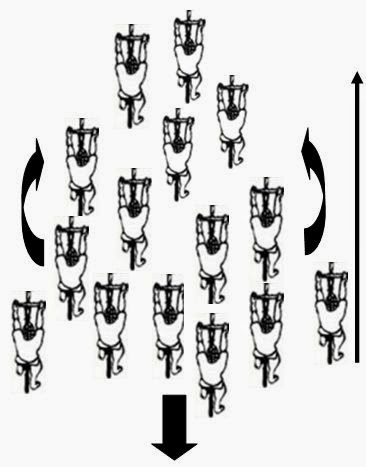
Figure 1. Illustrating the convective dynamic. Cyclists advance up peripheries (curved arrows), while riders in central region drift effectively backward (short thick arrow). Long arrow indicates direction of motion.

             In his paper [3], Erick Ratamero demonstrated a Netlogo agent-based model that simulated this convective effect in bicycle pelotons. From the perspective of clearly showing the collective vector pattern formation, Ratamero's simulation is extremely helpful. However, empirical data that clearly demonstrates this effect has still not been documented. The collective pattern formation of the cyclists in Video 1, for example, will have a sinusoidal appearance, which we know by tracking the trajectories of the simulated cyclists in Ratamero's model, as shown in Figure 2.

Figure 2. Sinusoidal pattern of simulated peloton of 100 cyclists in convective motion, applying method in [1] to quantify collective motion, and using Ratamero's MOPED peloton model [3]. Y-axis shows relative positions of each cyclist to all cyclists in the group.  X-axis is time. 

             Recently, I have purchased the rights to video footage of a stage of the Volta au Algarve, a professional bicycle stage race in Portugal. The footage is due to arrive any day now, and I am told it contains 1 hour of continuous overhead helicopter footage. I am optimistic the footage will show long-duration periods of the sort of behavior in Video 1 and that it will be sufficient to clearly establish the convective effect by applying the method of showing positional change as set out in [1].

            It is my objective also to demonstrate that this effect occurs in many multi-agent systems, including flocks, herds, and schools, and other biological collectives. 

            It seems that in order to establish that the principles underlying this effect are indeed self-organizing and naturally occurring (i.e. not an artifact of top-down human design, or simply a result of cyclists' racing strategy), it would be useful to demonstrate that the effect occurs in analogous systems which involve zero motivational influence; i.e. human motivations. Ideally, however, in order to isolate the pure physical principles that underlie the convective dynamic, we would go so far as to exclude even other animal systems in which individuals may also have strategic biases or motivations, and to seek analogous non-biological systems, if they exist or could be established by experimental design. 

           Such a non-biological system would involve purely physical forces, including a drafting effect that couples the system of particles or agents, a force to drive the collective in uni-directional motion, and some force that allows particles/agents from behind to move in a trajectory that allows for the hypothesized continuous convective motion. Barring a non-biological system like this, we may like to find analogous collective behavior among biological collectives that have minimal or no faculty to make volitional decisions, and whose motions are governed by very simple mechanisms, like bacteria or sperm, for example.

           Recently, I came upon this paper by Fortes, A., Joseph, D., and Lundgren, T. Nonlinear mechanics of fluidization of beds of spherical particles (1987) [4]. The authors describe experiments they did that demonstrate interesting two-dimensional dynamics of spheres in water. The authors used the apparatus shown below, which I have snipped and pasted directly from their published paper.  

Figure 3.  Image from the Fortes paper [4] of the apparatus they used.

            By dropping spheres from the top of the apparatus, the authors demonstrate a "drafting, kissing, and tumbling" dynamic, in which spheres following behind others in the direction of motion accelerate briefly relative to the one ahead in the lower pressure zone behind a leading sphere.  This is the drafting dynamic. Below, I have snipped and pasted Figure 5 from the author's published paper.

Figure 4. Image from the Fortes paper [4], which reads "Figure 5. Drafting, kissing, and tumbling in the vertical two-dimensional bed. The mechanisms are not affected by the inclination of the bed. Re=650."

            The Fortes results are very promising from my perspective, and I may be able to demonstrate the analogous convective effect by using a non-biological system similar to the Fortes system. Of course, I would still like to see if the effect occurs in bacteria and sperm and other similar systems, as this does not seem to have been documented. Nonetheless, if we have a drafting effect among falling spheres in water, we have two of the main force considerations that I think are necessary to demonstrate a convective effect: forward motion (here, induced by gravity), and an attractive force by drafting. 

            My hypothesis is that a small modification to the Fortes et al. apparatus may allow for a set of spheres to tumble two-dimensionally in a convective fashion. The modification I want to try is to curve the apparatus bed laterally. This curve will need to be sufficient to allow spheres to tumble past others and be forced to the peripheries of the group, and then to fall inward toward the bottom of the curve. It seems likely the effect, if it occurs at all, will only occur at the appropriate threshold apparatus angle and bed curvature. The angle and bed curve will dictate the collective sphere velocity, their corresponding drag reduction by drafting, and their relative acceleration at the front of the group toward the bottom of the curve. The reduction in drag due to drafting will, it seems, have to be sufficient to offset the loss of velocity in moving up the curve laterally, while the acceleration down the curve toward the front of the group will have to be greater than the velocity of those spheres rolling down the middle at the bottom of the curve.

           This bed curvature replicates a natural inclination for cyclists at the head of a group to gravitate toward a laterally central position (assuming no cross-wind). To show this position, in Figure 1 note the rider at the very top of the image - this rider would be in the "lateral center" of the race course.  It is not uncommon for more than one such "lateral center" to occur, each being offset from the center obviously, but well away from the edges of the course.

           I suspect that riders tend to gravitate toward this laterally centralized position at the head of the peloton because the lateral center represents physically the safest region between the lateral boundaries of the course; allows maximal peripheral view; multiple options for a line in which to drop backwards if so chosen; maximal options to adjust motion in response to passing movement from behind; and represents the most efficient position ahead of any curves in the road ahead. It will also be interesting to observe how this occurs in other flocking systems, as one suspects this formation is a universal self-organized one. 

          I have prepared a preliminary version of such an apparatus bed as discussed, shown in Figures 5a and 5b. The lateral curvature is shown in the left-hand image (albeit only in small degree) and the spheres at the bottom of the apparatus are shown in the right-hand image. However, the curvature needs to be modified and other modifications to the apparatus are required to make experimentation more efficient.  

         

Figures 5a and 5b. The proto apparatus for replicating the convective effect in a system of falling spheres in a viscous fluid. Figure 5a shows my attempt at forcing the bed to curve laterally.  Figure 5b shows the spheres at the bottom of the apparatus in a laundry soap fluid.  

           Since the apparatus requires modifications, I cannot of course report any results at this stage. Perhaps it will be entirely a bust, I do not know at this time.  However, I have been much inspired by the Fortes paper. In addition to this, I will be looking forward to analyzing the footage from the Volta au Algarve race, although that may take me all summer to do.

References and notes

[1] Trenchard, H., Richardson, A., Ratamero, E., M. Perc. 2014 Collective behavior and the identification of phases in bicycle pelotons, Physica A, Vol 405, 1 July 2014, 92–103

[2] Trenchard, H. 2013. Peloton phase oscillations. Chaos, Solitons & Fractals,Vol 56, November 2013, Pages 194–201

*Home video-cam recording of a live broadcast on http:\\mypremium.tv; Eurosport T.V. I am not certain what race it is from. I have not obtained the rights to use this video. 

[3] Martins Ratamero, Erick. 2013. MOPED: an agent-based model for peloton dynamics in competitive cycling. In: International Congress on Sports Science Research and Technology Support, 2013, Vilamoura, icSPORTS 2013, 2013.

[4] Fortes, A., Joseph, D., Lundgren, T. 1987. Nonlinear mechanics of fluidization of beds of spherical particles J. Fluid Mechanics, vol 177, p 467-483